SQL for the 21st Century: Analytic / Window Functions

I’m writing this blog post because the majority of SQL users is stuck in the past century.

It sounds like quite a bold statement. Let me start with why I think so.

Sometimes I interview candidates for positions that require some SQL literacy. I use an exercise that may lead to a complex SQL query involving many joins, self-joins, temporary tables, and aggregations.

Honestly, I have never expected anyone to put it together on the spot in 10 minutes. But it usually gave me 10 minutes of observing how the candidate thinks about the data.

Even though SQL window functions were officially introduced in the SQL:2003 revision of the SQL language, I rarely see a candidate think to use them in this kind of scenario. In fact, there was only one exception in last 5 years: Without losing a beat, the candidate said “I see, a window function” and in the next 30 seconds she sketched a more or less functional (and much simpler) query on the whiteboard.

So, for those of you who may not think to use one right away, what are window functions (also known as analytic functions) all about?

If you open a documentation of any SQL database, you will notice three types of functions:

• Single row functions (and operations): turn values in a single row into a new value (this is what the majority of SQL functions does)
• Aggregate functions: turn many rows into a single value (these are the functions that usually require the GROUP BY clause)
• Window functions (also known as analytic functions): this is what this blog post is about

Let me start with a few visual examples:

Row-level functions

Row-level functions (and operations) operate on individual rows. They may take columns of each processed input row as parameters and produce value that is included in the single output row.

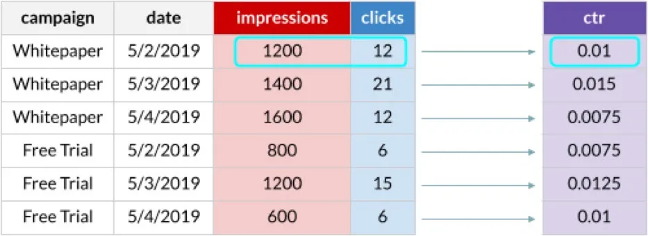
The result set from the diagram above can be created by the following simple query:

SELECT clicks / impressions as ctr FROM campaigns

In this example, we were using division. Besides arithmetic operations, other examples of row-level functions include mathematical functions, date functions, string functions, and many others.

Aggregate functions

Aggregate functions take a group of rows with a common set of values (identified by the GROUP BY clause) and turn them into a number.

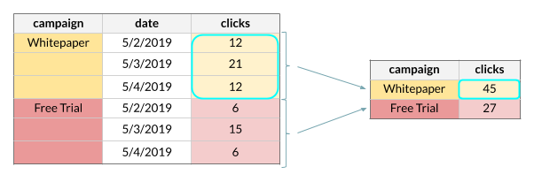
Common examples of aggregate functions include SUM, MIN, MAX, and AVG.

Window functions

Similarly to row-level functions, window functions process rows one by one and produce one output value for each input row.

Unlike row-level functions, window functions can split input data into partitions (or “windows” or “window frames” - hence the name) where a partition includes multiple rows that are somehow related to the currently processed row.

Let’s jump right into some examples.

Since you are probably familiar with aggregate functions, let’s start with their window-based counterparts. Meet aggregate window functions!

A picture is worth a thousand words:

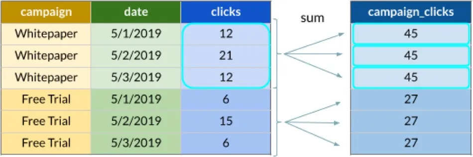
The full SQL for the table above is as follows:

SELECT
SUM(clicks) OVER (PARTITION BY campaign) AS campaign_clicks
FROM campaigns

Note: Other well-known aggregate functions such as AVG, MIN, MAX, COUNT, etc, can be used in the same way.

The OVER keyword defines the data windows; the PARTITION BY clause says that each campaign value represents a different window. It means the SUM aggregates clicks from all rows where the campaign is the same as in the currently processed row.

Just to illustrate, a comparable SQL without window functions would look like this:

Don’t do this!!!

SELECT a.clicks
FROM campaigns c
INNER JOIN (
  SELECT campaign, SUM(clicks) AS clicks FROM campaigns GROUP BY campaign
) a
ON c.campaign = a.campaign

It’s uglier, it’s longer. Moreover, window functions in general perform better than self-joins.

Intermezzo: Why window functions?

At a glance, it does not make much sense to repeat the same value for every row within a window frame.

The point is usually in combining window functions with additional logic. For example, the window SUM function can be used to easily compute a percentage of each row’s value to a bigger part.

In this example, a window function performs a calculation that is used to compute share of clicks for each day of the campaign:

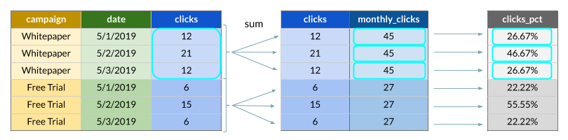
This is typically achieved by using a subquery with the window function like this:

SELECT clicks / campaign_clicks FROM (
SELECT clicks,
       SUM(clicks) OVER (PARTITION BY campaign) AS campaign_clicks
FROM campaigns
) q

As shown in this example, window functions typically don’t solve what one could call a “business problem.” They enable SQL users to solve many business problems using a shorter, more readable, and better performing code compared to alternatives typically involving aggregate functions and self-joins.

Ordered window frame: LEAD, LAG, FIRST_VALUE etc

Window definitions can define an ordering using the ORDER BY clause (optionally with the usual ASC and DESC modifiers).

An ordering can be used by the FIRST_VALUE (and LAST_VALUE) function with obvious meaning:

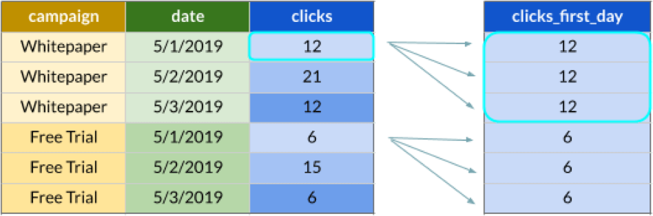
Now the SQL:

SELECT
FIRST_VALUE(clicks) OVER (PARTITION BY campaign <strong>ORDER BY</strong> date) AS clicks_first_day
FROM campaigns

The LAG and LEAD function that can bring value from the previous or next row given the window ordering:

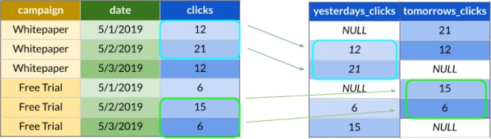
SELECT
LAG(clicks) OVER (PARTITION BY campaign ORDER BY date) AS yesterdays_clicks,
LEAD(clicks) OVER (PARTITION BY campaign ORDER BY date) AS tomorrows_clicks
FROM campaigns

Did you want to compute day-over-day changes? Here you go.

Ranking functions

Other ordering-related window functions are ranking functions such as ROW_NUMBER, RANK, and RANK_DENSE. Intuitively, they should do something with the position of each row of the query result within its window.

What do they do, and how are they different from each other? Again, let’s start with a diagram:

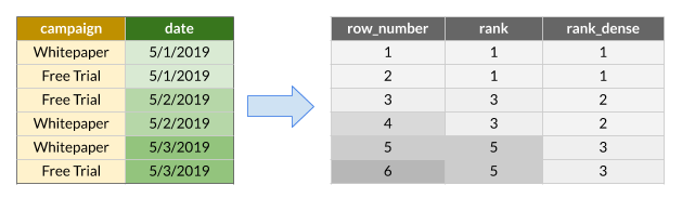
For a better visual illustration, we are demonstrating one more feature here: You can have only one partition that actually spans the entire result set; just omit the PARTITION BY clause from the definition of the partition.

Note it’s up to the database server to decide how it orders rows with the same date.

The result set includes the following columns (named after the corresponding functions):

• ROW_NUMBER: The number of each output row within a partition. Always unique. If two rows are equivalent with regards to the window ORDER BY clause, it’s up to the database engine to decide which goes first (and thus which will result into a smaller row number).
• RANK: Returns the rank of each row within the resulting partition. Unlike ROW_NUMBER, RANK outputs the same values for equally ranked rows. The rank is based on the number of previous rows, which means that equally ranked rows cause gaps.
• RANK_DENSE: Like RANK but denser. The rank is based on the number of previous distinct values of the sort column.

SELECT
 ROW_NUMBER() OVER (ORDER BY date) row_number,
 RANK() OVER (ORDER BY date) rank,
 RANK_DENSE() OVER (ORDER BY date) rank_dense
FROM campaigns

By the way, if you find the repeated occurrences of the window definition a little annoying, we have good news. This query can be rewritten using named windows so the window definition can be kept at a single place after the WINDOW keyword:

SELECT
 ROW_NUMBER() OVER all_campaigns_by_date row_number,
 RANK() OVER all_campaigns_by_date rank,
 RANK_DENSE() OVER all_campaigns_by_date rank_dense
FROM campaigns
WINDOW all_campaigns_by_date AS (ORDER BY date) –– named window

There are many applications for the ranking functions. For example, you can use them for row deduplication.

Imagine that our campaigns table holds all updates for each campaign and date. In this case, we may want to extract the last update for each campaign and date like in the following example:

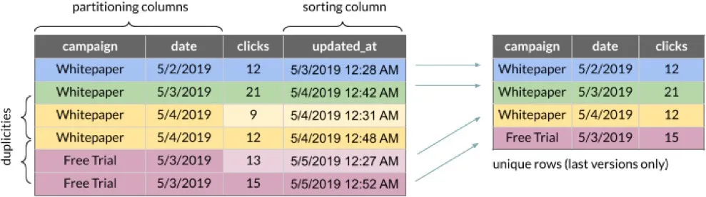
We can use the same technique as in previous examples: using a subquery with a window function to pick only the last version for each id:

SELECT id, campaign, date, clicks
FROM (
SELECT *,
  ROW_NUMBER()
    OVER (PARTITION BY campaign, date ORDER BY updated_at DESC) AS row_number
) q
WHERE row_number = 1

A kind reader may notice that there are more ways to achieve this goal. How about FIRST_VALUE or LAST_VALUE? Sure, it will work too.

Just please don’t use aggregations (GROUP BY) and self-joins or SELECT DISTINCT for this use case.

There is, however, one possible issue with this solution. Can you find it? Hint: It’s not about using the function right or wrong but more about understanding the business context.The right answer is at the end of the article.

Window frame clause and running totals

So far our examples were using static partitions. This may be limiting for some use cases that would otherwise look like clear applications of window functions.

For example, running totals. In our previous examples, we knew how many clicks each campaign generated each day, and how many clicks it generated in total. How about clicks-to-date?

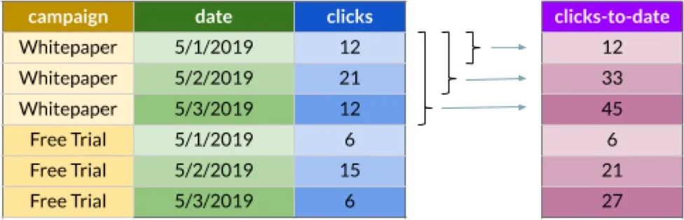
SQL:2003 provides so-called window frame specification keywords or window frame clauses for this kind of problem:

SELECT
SUM(clicks) OVER (PARTITION BY campaign
                  ORDER BY date
                  ROWS BETWEEN UNBOUNDED PRECEDING AND CURRENT ROW)

The last line starting with ROWS does the job.

Yes, we don’t want to sum all clicks from each campaign-specific partition. Instead, with regards to the ordering (ORDER BY date), we only want to include a subset of partition’s rows. Specifically, only the rows from the first one within the partition up to the current row. The code reads itself, doesn’t it?

The structure of the window frame specification starting with the ROWS keyword is as follows:

ROWS BETWEEN <start-point> AND <end-point>

The start-point can be one of the following:

• UNBOUNDED PRECEDING specifies all rows from the beginning of the sorted partition until the end-point
• <number> PRECEDING includes the <number> of rows before the current row
• CURRENT ROW is obviously the current row

For the end-point specification, the following keywords work in a similar way:

• UNBOUNDED FOLLOWING
• <number> FOLLOWING
• CURRENT ROW

For example, do you want to sum all rows within a partition starting from 2 rows before the current one until the end of the partition? Not sure why would anybody do that but if it solves your problem, try ROWS BETWEEN 2 PRECEDING AND UNBOUNDED FOLLOWING.

You can sometimes see terms such as cumulative window frame and sliding window frame. Cumulative frame includes the UNBOUNDED start or end point, while the sliding frame uses a combination of CURRENT ROW and <number> FOLLOWING or PRECEDING

Year-to-date

If you think about it, year-to-date is just a special case of the previous example where the data is partitioned by year:

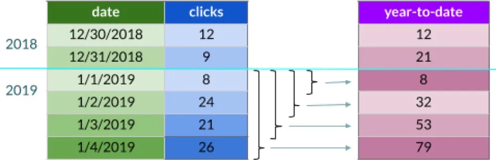
The corresponding SQL can be left as homework for a kind reader. Select the following text to reveal the answer:

SELECT
SUM(clicks) OVER (PARTITION BY YEAR(date)
                  ORDER BY date
                  ROWS BETWEEN UNBOUNDED PRECEDING AND CURRENT ROW)

ROWS vs. RANGE and time windows

SQL:2003 provides two ways of fine tuning which rows from each partition should be included in each row-specific window frame.

The previous example introduced the ROWS keyword. For ordered partitions, it can be used to limit the window frame by rows.

Sometimes you prefer to limit window frame by value. For example, when processing time series data, you want to restrict the window frame to from ten minutes before the value to the value in the currently processed row (which may theoretically include not yet processed rows containing the same value!).

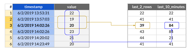
Note the timestamp in row #4 is the same as in row #3. This is why row #4 belongs to the range between row #3 and 10 minutes ago.

SELECT
SUM(value) OVER (
  ORDER BY timestamp
  ROWS BETWEEN 1 PRECEDING AND CURRENT ROW) AS last_2_rows,
SUM(value) OVER (ORDER BY timestamp
  RANGE BETWEEN ‘10 minutes’ PRECEDING AND CURRENT ROW) AS last_10_minutes
FROM my_table

The bad news is that RANGE is not a widely supported feature. Many major database engines don’t support sliding ranges (i.e. the RANGE keyword with <number> PRECEDING or <number> FOLLOWING). Even worse, some of them do not support RANGE at all. Please check the documentation of your database engine first.

Combining window functions and GROUP BY

Sometimes you may want to combine the output of a window function with good old aggregation functions and GROUP BY statement. Maybe something like this:

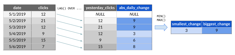
The SQL syntax does not allow you to combine these two within a single simple query but it can be easily worked around using subqueries.

For example, the type of calculation outlined in the diagram above can be easily addressed by the following code:

SELECT MIN(ABS(clicks - yesterday_clicks) AS smallest_change,
      MAX(ABS(clicks - yesterday_clicks) AS biggest_change
FROM (
SELECT clicks,
       LAG(clicks) OVER (ORDER BY date) AS yesterday_clicks
) q

Commercial break: Why are we talking about SQL?

Put simply: we love SQL. It’s a great tool for transforming data, and it’s the lingua franca for data engineers—regardless of what other tools or languages they may use.

For example, even though GoodData is known for its use of a high-level analytic query engine MAQL on top of a semantic layer, that analytic engine still translates reusable insight definition elements into effective SQL statements. Customers also have the option of using our data pipeline tooling to orchestrate the flow of SQL transformation, possibly even with our hosted data warehouse based on Vertica (and yes, it fully supports RANGE).

But however much we love SQL, we also believe there is a better way when it comes to building the last mile of an analytic solution (Take a look at our recent blogpost on what modern analytics really is for more).

That’s why our platform gives solution creators a semantic layer built for today’s complex data that is both easy to learn and ensures reusability and agility.