Least-Squares Functions
The least-squares method of linear regression attempts to fit a linear regression trend line as closely as possible. This line has the smallest possible value for the sum of the squares of the errors between the predicted value of the line and the actual two-dimensional data points.
In the following diagram, the least-squares linear regression plots a line through the set of points that minimizes the sum of the squares of the error factors.
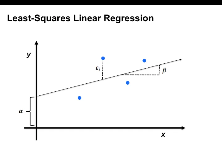
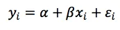
The actual data points are calculated using the following equation:
Use the R-squared function (RSQ) that returns square of the correlation coefficient to measure how well the linear regression expresses the variability of the Y values around their mean.
RSQ (*numeric1*, *numeric2*)where numeric1 and numeric2 are facts or metrics
Computes the R-squared value for the two sets of numeric values. Also known as the coefficient of determination, R-squared ranges between 0 and 1, with a value of 1 indicating that the model explains all variability in the dependent variables data.
R-squared does not determine if there is bias in the estimates.
Syntax
SELECT RSQ(metric1, metric2)
SELECT RSQ(fact1, metric2)
SELECT RSQ(fact1, fact2)
Examples
SELECT RSQ({metric/count_of_defects}, {metric/production_volume})