Many-to-Many in Logical Data Models
During a typical multidimensional analysis, every dimension attribute participates in a simple one-to-many relationship with every fact. Design of the model then follows a star or a snowflake schema.
In more complex models, multiple stars/snowflakes exist. Users are guided during analysis and only relevant dimension attributes connected via one-to-many relationships are offered. This provides a safe and intuitive environment for the analyst.
The real-world complexity sometimes requires analysis over many-to-many relationship, also known as M:N. The following sections give you information on how to prepare your logical data model for these more complex use cases.
Set up M:N relationships in LDM
Let us demonstrate the many-to-many relation on the following example with projects and consultants:
| Project | Revenue | Consultant |
|---|---|---|
| alpha | 8,000 | Alice |
| Joe | ||
| beta | 18,000 | Bob |
| Cath | ||
| Joe | ||
| gamma | 33,000 | Bob |
| Cath | ||
| Ed | ||
| Jim | ||
| delta | 12,000 | Alice |
| Cath | ||
| Ed |
The many-to-many relationship between Project and Consultant in this example means that one consultant works on multiple projects and multiple consultants work on one project.
Analytics should be able to provide answers, for example, to the following questions:
What is the revenue per project where Cath works?
What is the total revenue from projects where Alice works?
How many consultants work on each project?
To answer all the questions we need to model data differently in a relational model.
You can create separate entities for Project and Consultant, and capture their relation in a bridge dataset named Timesheet.
You can calculate Revenue in our example from fact Amount of dataset Invoice using the following formula: SELECT SUM(Amount)
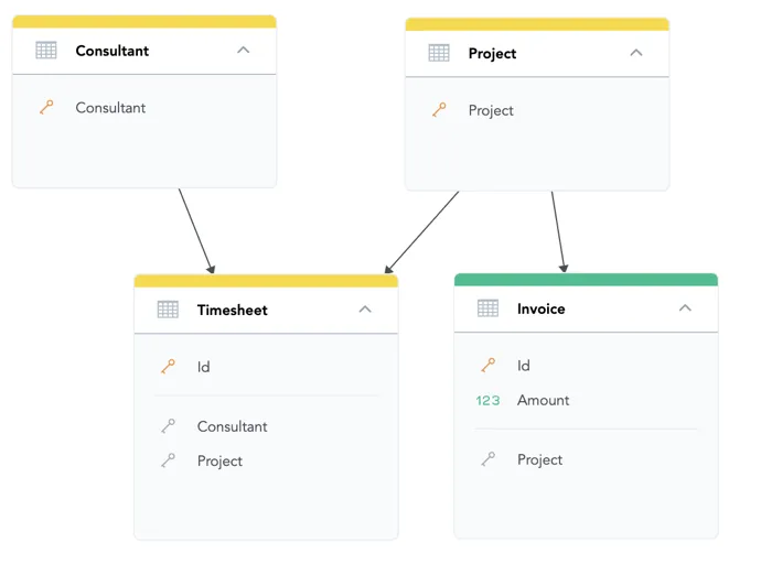
To break down the Revenue metric by an attribute from which an oriented path to the fact Amount exists.
You can use the Project attribute in the Project dataset, or the Id attribute in the Invoice dataset.
You cannot use any attributes from the Consultant or Timesheet datasets.
The engine treats the Timesheet dataset as a center of a different star than the star with Amount.
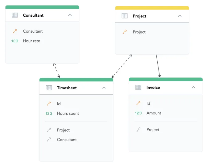
To help the query engine recognize the Timesheet dataset as a bridge dataset of many-to-many relationship and differentiate it from ordinary datasets, drag an arrow from the Timesheet dataset to the Project dataset.
This many-to-many edge in the logical data model is indicated by a two-sided arrow (see the image below).
The filled arrow points in the original direction of one-to-many relationship between Timesheet and Project.
The empty arrow indicates that this relationship can be used to connect a part of the logical model over the many-to-many relationship from the bridge to the rest of the model.
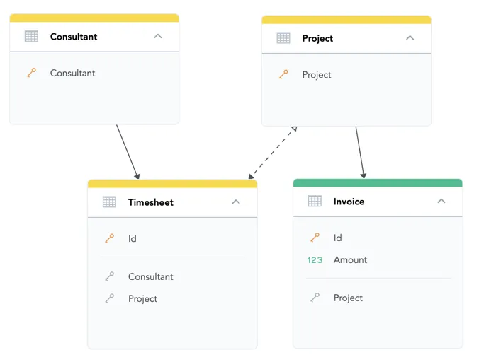
You can now calculate Revenue from Amount on Invoice and filter it or break it down by any attribute in the data model because an oriented path from each dataset to the Invoice dataset exists.
Double Counting with M:N
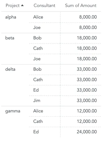
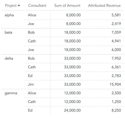
When you slice the Revenue by both the Project and the Consultant attributes, you will see the effect of double counting:
The Revenue for the Alpha project repeats for each consultant working on this project.
Also, hours that Ed spent on the Gamma project are split into two timesheets. The total revenue for the Gamma project is only 12,000, you see 24,000.
Sum of all rows in the table is higher than the total revenue from all projects.
To avoid this effect of double counting when using attributes over many-to-many relationships, use the technique called allocation factor.
Allocation factor
In the Timesheet bridge dataset, add the Hours spent fact. This will allow you to allocate the calculated revenue to consultants proportionally based on their allocation (i.e., the number of hours spent on a project).
The formula for Attributed Revenue must take the allocation factor into account and weight the revenue of consultants on the projects by their contribution:
SELECT SUM({fact/amount} * {fact/hours_spent} / (SELECT SUM({fact/hours_spent}) BY {label/project}))
This formula:
Multiplies the Amount from the Invoice table by Hours spent from the bridge dataset Invoice.
Divides it by the sum of all Hours spent on a project (the same value is used in all rows belonging to the same project).
Other example of using facts stored in a bridge dataset is currency conversion - you can use many-to-many relation to convert value from a fact table into a selected currency.
More complex models
Models with a single many-to-many edge (double-sided arrow) are suitable for asymmetric use cases - they let you cross the many-to-many bridge dataset only in a single direction.
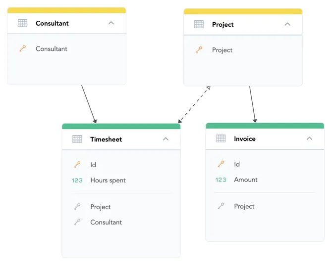
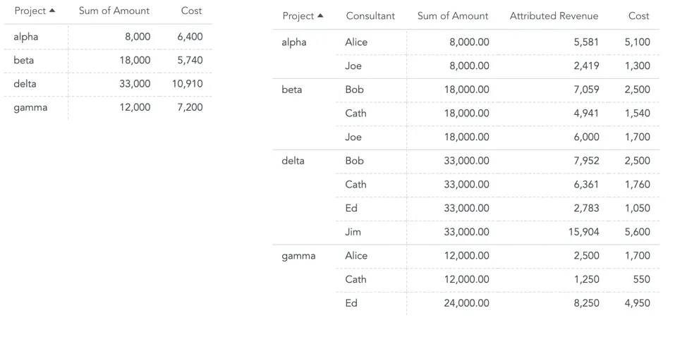
The following model shows a complex use case where the Consultant dataset also contains information about the Hour rate of consultants.
The Hour rate allows you to compute the costs of a project. You must add an additional may-to-many edge between Timesheet and Consultant to create an oriented path from the Project dataset to the Consultant dataset via Timesheet.
The formula for the Cost is: SELECT SUM({fact/hour_rate} * {fact/hours_spent})
Limitations to M:N
Allowing many-to-many relationships in your logical data model requires careful planning. You want to avoid ambiguity in how the GoodData engine interprets the relationships and approaches calculations.
The following data model schemes show the NOT-recommended modelling structures among datasets.
Alternative paths
The following model is valid, but you need to be aware how the alternative paths are resolved.
The analytical engine selects the shortest path in any computation (A → B).
You can set one of the paths as many-to-many, since there is only one shortest path.
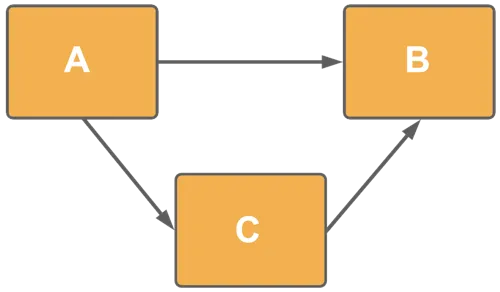
Alternative paths with many to many
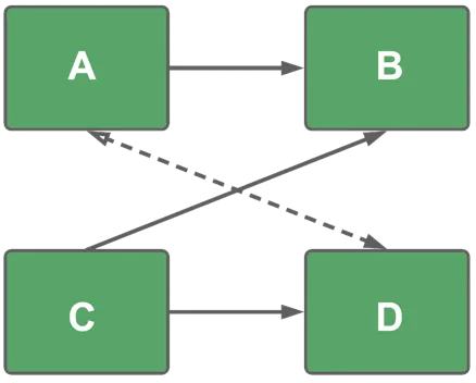
There are alternative paths (C → B and C → D → A → B), but the analytical engine will select C → B because it is the shortest path.
Ambiguous paths
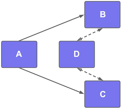
Two or more paths have the same length: A → B → D or A → C → D. The analytical engine selects one path randomly.
Negative filters results when used in M:N model
The syntax WHERE Attribute NOT IN (values) returns records where the result includes at least one different value from the filtered value. You can also use WHERE NOT Attribute IN (values) for the same results.
Analytical Designer generates NOT ( [attribute] IN ( [element1, element2, ...] )) for negative filters.
| Project | Consultant |
|---|---|
| alpha | Alice, Joe |
| beta | Alice |
| gamma | Joe |
| delta | NULL |
Queries and results for `View By: Project`
| Query | Result |
|---|---|
WHERE {label/Consultant} IN ("Alice") | alpha, beta |
WHERE {label/Consultant} = "Alice" | |
WHERE {label/Consultant} NOT IN ("Alice") | alpha, gamma |
WHERE {label/Consultant} <> "Alice" | |
WHERE NOT {label/Consultant} IN ("Alice") | |
WHERE NOT {label/Consultant} = "Alice" | |
WHERE {label/Consultant} NOT IN ("Alice", "Joe") | no result |
WHERE NOT {label/Consultant} IN ("Alice", "Joe") |